Introduction
The swin transformer is proposed because the previous transformer has the following two shortcomings in the field of visual processing:
- Unlike NLP, the pixel resolution of an image is much larger than that of text information. If pixels are used as tokens, the computational complexity is unacceptable.
- The objects in the image often have different scales, which is also not effectively handled by the previous viT, such as: instance segmentation in densely predicted scenes.
In order to solve these problems, swin transformer has proposed some new solutions.
This blog mainly focuses on the following aspects:
- Patch Merging
- Window Self-Attention
- Shift Window Self-Attention
- Relative Position Index
And as repeatedly emphasized in the paper, the swin transformer not only solves the above two problems, but more importantly, the author proposes a general-purpose backbone network, although the performance of the unified model in the NLP and CV fields is not as good as viT, but Its future development is worth looking forward to.
NOTICE: Reading this blog requires a basic understanding of viT.
Patch Merging
As mentioned above, viT does not handle the problem of image multi-scale very well. Looking back at CNN, when dealing with multi-scale problems, we have a good method: FPN.
So how do we apply this idea to transformers? The author proposes Patch Merging. Simply explained, this is to achieve the CNN effect with a non-CNN method.Continuing to read the paper, we will find that the author built the network with the effect achieved by CNN as a template.
First, in terms of scale, the comparison between swin transformer and viT can be seen in the following figure: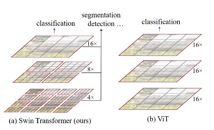
From the above figure we can see that the scale of the swin transformer increases step by step compared to the single scale of viT ($ 16 \times 16 $). With each increment, the feature map size is halved and the number of channels is doubled, which is very similar to CNN.
That is to say, the patch size at the beginning is $4\times 4$, followed by $8 \times 8$,
$16 \times 16$, and the receptive field is getting bigger and bigger, forming multiple scale.
Then we look at the structure of the entire network: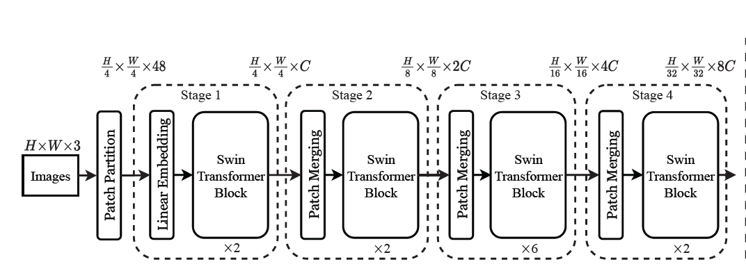
If the input image is a 3-channel image, the size is $H \times W$, after the first layer, the
scale is reduced to 1/4, and the number of channels becomes $4\times 4 \times 3 = 96$, after the first layer stage, the scale remains unchanged, and the number of channels becomes C, where C depends on the size of the model, as shown in the following figure. After each stage, the scale is reduced by half and the number of channels is doubled.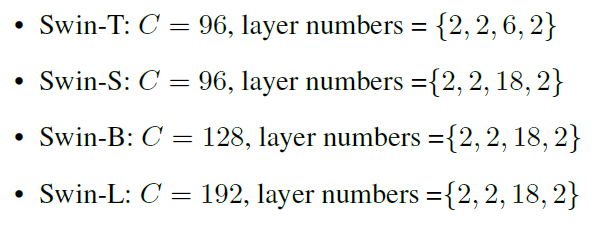
Notice: Patch Partition + Linear Embedding in the figure has a similar effect as Patch Merging.
Detail of Patch Merging
Now we know what Patch Merging does, but how does it work? Next I will use a simple example to illustrate.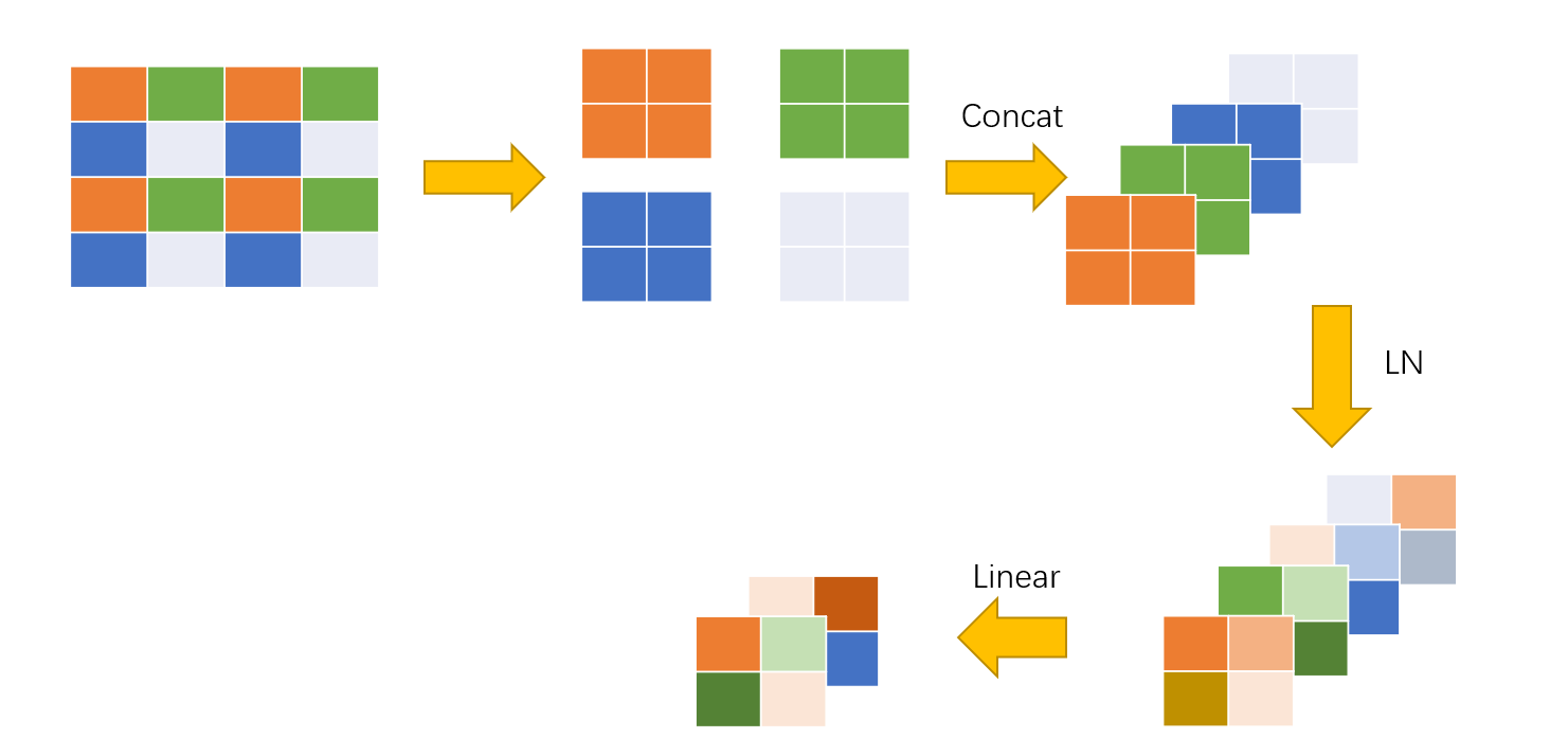
Here we have a feature map of $4 \times 4$, take a single channel as an example, divide it into 4 windows, take the patches at the same position in each window (marked with the same color here), and merge them to increase the number of channels, Then LayerNorm is performed, and finally a linear operation is performed to halve the number of channels. This is the whole process of patch-merging, which realizes the operation of halving the scale and doubling the number of channels.
Window Self-Attention and Shift Window Self-Attention
For the computational complexity mentioned above, the paper uses a window self-attention model. In order to connect different windows and achieve a global approach, a shift window self-attention model is proposed.
Take this picture in the paper as an example: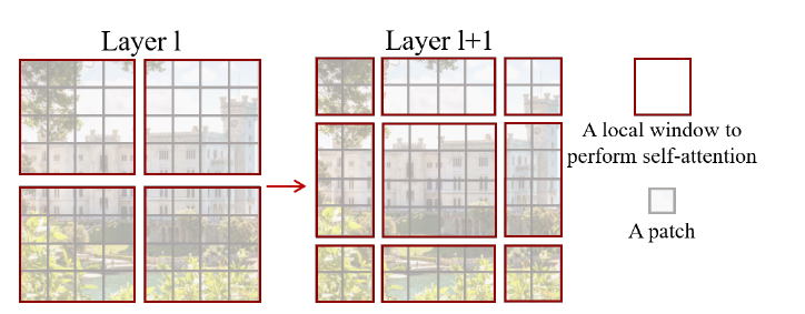
Window Self-Attention(W-MSA)
First look at the following figures. The entire image has $8\times 8$ patches, divided into 4 windows, each window has $4\times 4$ patches.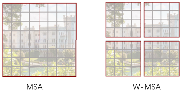
If we use MSA, such as the left picture, we have to calculate the self-attention of one patch with all other patch, and if we use W-MSA, we only need to calculate the self-attention of each window. As the scale of the feature map increases, MSA is a squared increase, while W-MSA increases linearly.
The paper gave the calculation-functions for these two methods: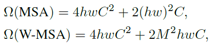
Parameter Description:
- h: height of feature map
- w: the width of the feature map
- C: the number of channels of the feature map
- M: size of a single window
Additional Part(Computational complexity)
This part is an additional part to explain how the above complexity calculation formula comes from.
Here we use FOLPs as the metric, and first we need to know the FOLPs of the matrix calculation. Such as $A^{m \times n}\times B^{n \times v}$, the FOLPs is: $m \times n \times v$.
Review the calculation of Attention:
For each patch in the feature map, the corresponding q, k, v are generated through $W_q, W_k, W_v$,
It is assumed here that the vector lengths of q, k, v are consistent with the depth C of the feature map. Then the process of generating Q for all patches is as follows:
The FOLPs is: $hw \times C \times C$, the same as K and V, with total of $3hwC^2$.
And the is $Q K^T$, the FOLPs is $(hw)^2C$, then ignore division by $sqrt{d}$ and $softmax$,
and finally, multiply by V, so we can obtain the following FOLPs:
Finally is the matrix about mutil-head $W_o$, the FOLPs is $hwC^2$.
So we get: $4hwC^2+2(hw)^2C$
For W-MSA, we can also get the function with a similar calculation process.
Shift Window Self-Attention
Now comes the part that I think is the most interesting.
Although we significantly reduce the computational complexity through windowed self-attention, it also creates a problem: global information is lost. We only focus on attention within a window, and there is no connection between windows.
To solve this problem, the author proposes a new method: Shift Window Self-Attention. As shown below:
After finishing the W-MSA on the left, we shift the image a few patches to the right and down, this amount of “Shift” depends on $\frac{|M|}{2}$, and then divide the image again.
In this way we can connect patches that were not in the same window before. But this creates a new problem: as shown on the right, the new feature map has 9 windows. If they are calculated separately, their sizes are different and cannot be calculated uniformly. If padding is used here to expand it to the same size, the self-attention of 9 windows needs to be calculated, which increases the computational complexity.
In order to unify the self-attention of the calculation window without increasing the computational complexity, the author proposes an interesting method: cyclically shift the window to achieve unified calculation and reduce the computational complexity.
As shown below: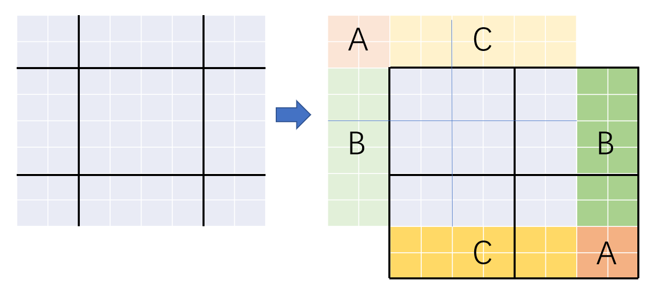
We spliced parts A, B, and C separately, taking the middle window as an example, after shifting, it can contact the original 4 windows.
But now a new problem has arisen. Although this method can keep the computational complexity from increasing, the window formed by shifting and splicing will cause errors if we directly calculate self-attention. Since they have moved from far away, the connection between the two should be minimal.
For example, if “C” stands for “sky”, we concatenate it with “ground” below, and the calculated self-attention is obviously inappropriate.
To avoid this error, the authors propose a new masking method.
Regarding this method, the author gave a detailed explanation in issues #38 in his GitHub, as shown below: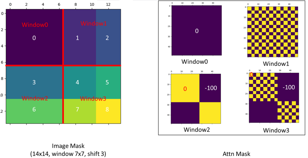
That is to say, in the required position, the mask value is 0, and in the unwanted position, the value is -100. Since the value after self-attention calculation is very small, after subtracting 100, through softmax, in the unwanted position, the value will approach 0 indefinitely.
Finally, after the calculation, it is necessary to restore the shifted part back to its original position.
Relative Position Index
This part belongs to the optimization part of the project and is not required, but it can improve the performance of the model(as shown below).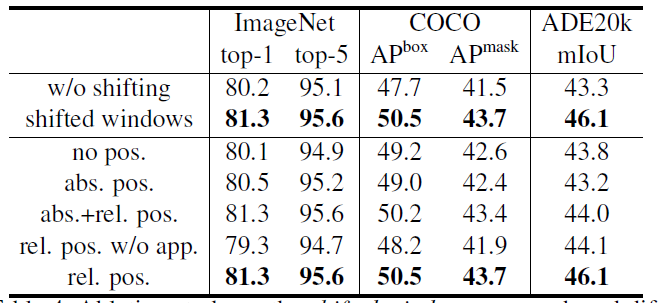
The process of building a relative position index is as follows:
Step 1: Build a relative position matrix based on each patch, flatten, merge.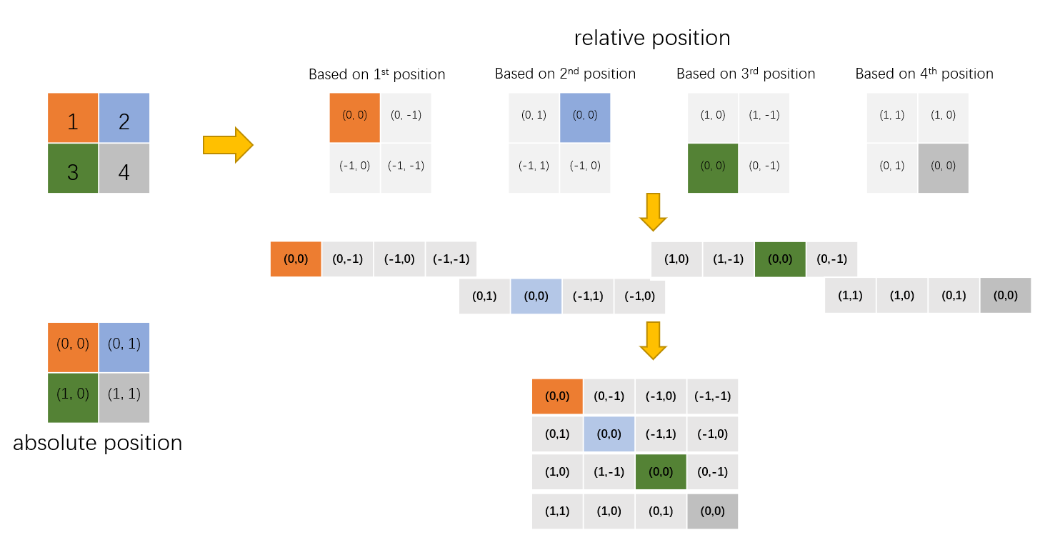
Step 2: The simple relative position index has actually been completed, but in the source code, in order to express more concisely, each index is represented by one-dimensional rather than two-dimensional coordinates. But how? If we directly add the two-dimension coordination together, then (0, -1) and (-1, 0) will have the same value.
In order to avoid this problem, author use the following method:
Add M-1 to the original relative position index (M is the size of the window, in this example M=2), after adding, there will be no negative numbers in the index.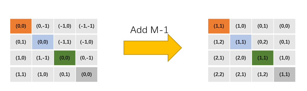
Step 3: Then multiply all row values by 2M-1: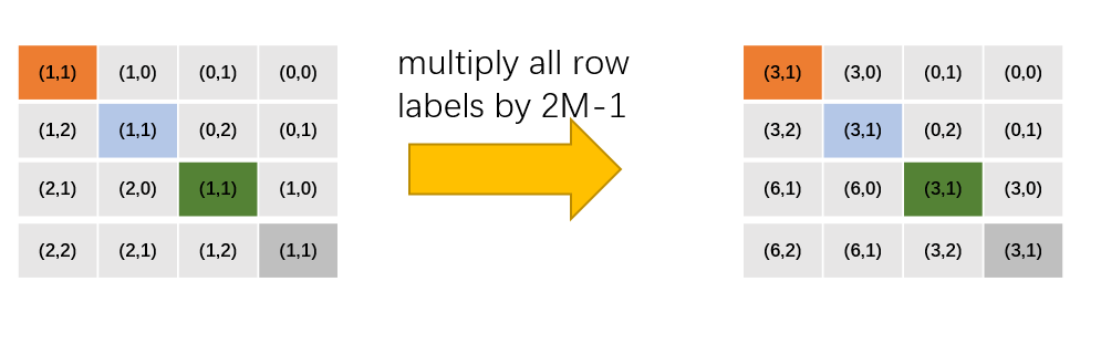
Step 4: Add row and column values: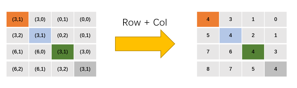
Step 5: Finally get the value according to the index: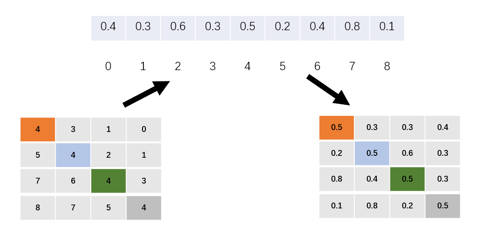
Now the process of relative position index and value is completed.